Can We Predict a Biogas Bi-Reforming Reactor from First Principles?

Can We Predict the Reactor Before We Build It?

Imagine that we want to design a biogas bi-reforming reactor before we actually build it. We know what will enter the reactor: methane, carbon dioxide, and steam. We know which catalyst we want to use, how large the reactor may be, what pressure it will operate at, and how heat will be supplied. At first, this sounds like a problem that modern engineering should already know how to solve. The laws of mass, energy, and chemistry are known, computers are powerful, and we already have decades of research on catalytic reactors. So we should be able to calculate what comes out if we know what goes in. We would like to predict methane conversion, hydrogen production, the H₂/CO ratio, the temperature inside the catalyst bed, pressure drop, the chance of carbon formation, and perhaps even how the reactor will behave after hundreds or thousands of hours. We would also like to make these predictions before seeing experimental results, rather than changing model parameters afterward until the calculation agrees with the experiment. If we could do this reliably, the model would become a true reactor-design tool rather than simply a way to reproduce something we already measured. Everything inside the reactor is made of atoms and molecules that obey physical laws, so somewhere between the inlet and outlet, the answer must exist. The interesting question is not whether we can write equations for the reactor, because we certainly can. The real question is how far those equations can take us before we need information that physics alone cannot give us.

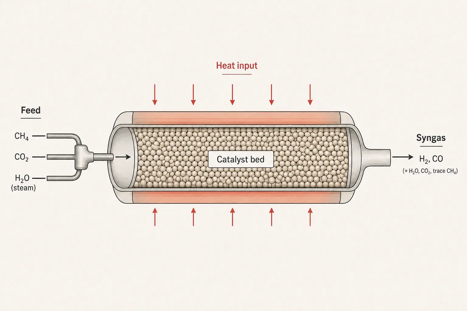
Figure 1 makes the reactor look almost simple. Methane, carbon dioxide, and steam enter from one side; a catalyst bed sits inside a heated tube; heat enters through the wall; and hydrogen-rich syngas leaves from the other side. That simple picture is useful because it gives us a starting point without forcing us to think about everything at once. We can now begin with the easiest question: if the gases were allowed to react for a very long time, what final chemical mixture would they prefer to reach? This question does not require us to know the reactor length, the pellet size, or how fast the gas flows. It is mainly a question of thermodynamics. In biogas bi-reforming, several reactions occur together, but three reactions give us a useful starting picture. Steam reforming uses methane and steam, dry reforming uses methane and carbon dioxide, and the water-gas shift reaction connects carbon monoxide, steam, carbon dioxide, and hydrogen. These reactions do not happen independently because changing one species changes the conditions for the others. Temperature also changes which direction each reaction prefers, while pressure and feed composition shift the final chemical balance. Before worrying about how fast anything happens, thermodynamics tells us what final state is possible. That already gives an engineer useful information because there is little value in designing a reactor for a chemical result that thermodynamics does not allow.

Where Does the Chemistry Want to Go?

Steam methane reforming can be written as:

$$\mathrm{CH_4 + H_2O \rightleftharpoons CO + 3H_2}$$

Dry reforming can be written as

$$\mathrm{CH_4 + CO_2 \rightleftharpoons 2CO + 2H_2}$$

The water-gas shift reaction is:

$$\mathrm{CO + H_2O \rightleftharpoons CO_2 + H_2}$$

These three short equations hide a surprisingly complicated chemical system. Methane can react with steam or carbon dioxide, while carbon monoxide, hydrogen, steam, and carbon dioxide continue to interact through the water-gas shift reaction. This means that changing the amount of steam does more than change methane conversion; it can also change the H₂/CO ratio, carbon formation tendency, and total heat requirement. Changing temperature affects both the reforming reactions and the water-gas shift reaction, so the outlet composition can move in several directions at once. Thermodynamics helps us calculate the chemical balance that the system approaches when enough time is available. At equilibrium, the reaction no longer has a net tendency to move further in one direction, and the Gibbs free-energy change becomes zero. The useful connection between Gibbs free energy and the equilibrium constant is the following:

$$\Delta G_r^\circ=-RT\ln K_{\mathrm{eq}}$$

The equation may look formal, but its message is simple: temperature and thermodynamic properties tell us how strongly a reaction prefers products or reactants at equilibrium. With good thermodynamic data, we can estimate equilibrium methane conversion, syngas composition, and whether solid carbon is thermodynamically favored under a chosen operating condition. We can also explore how changing temperature, pressure, steam content, or CO₂/CH₄ ratio moves the possible reactor outcome. For a moment, this feels like we are already close to predicting the reactor.

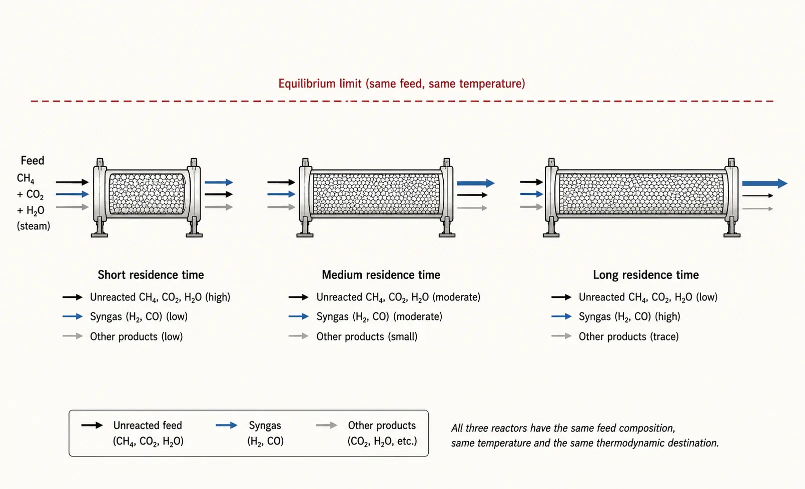
Figure 2 shows why we are not finished. The three reactors have the same feed and the same temperature, so thermodynamics gives them the same final equilibrium limit. Yet the short reactor may leave much more methane unreacted, the middle reactor moves closer to equilibrium, and the longer reactor may get closer still. Nothing is wrong with the thermodynamic calculation. The problem is that thermodynamics does not know how much time the gas has spent inside the reactor. It tells us where the chemistry wants to go, but not how quickly it can get there. A gas mixture that would eventually reach high methane conversion may leave the reactor much earlier because it only spends a small amount of time over the catalyst. The same chemistry can therefore produce different outlet compositions simply because reactor length or flow rate changed. This is the first important limit of the simple model. We now need something that gives chemistry a clock. That something is reaction kinetics. Once kinetics enters the problem, we can begin asking how much reaction occurs in one second, two seconds, or any other residence time. We are no longer asking only where the system can end up; we are asking how fast it moves toward that point.

Giving the Reactor a Clock

A common starting point for reaction kinetics is the Arrhenius equation:

$$k=A\exp\left(-\frac{E_a}{RT}\right)$$

Here, (k) is the reaction-rate constant, (T) is temperature, (E*_a*) is the activation energy, (R) is the gas constant, and (A) is a fitted or estimated factor. The most important part for a reader to understand is that reaction rate can change very strongly with temperature. A reactor that is only moderately hotter can sometimes react much faster because the temperature appears inside an exponential term. This is one reason temperature control is so important in catalytic reforming. Real catalytic kinetics, however, are usually more complicated than a single Arrhenius equation. Methane, steam, carbon dioxide, hydrogen, and carbon monoxide may compete for locations on the catalyst surface, and products can slow or reverse some reaction steps. Engineers therefore often use rate equations that include adsorption, reaction, and equilibrium effects. These equations can become quite detailed, but that is not the important issue here. The more important question is where the kinetic constants came from in the first place. Some may come from experiments, some from molecular calculations, and some from fitting a model to measured reactor data. Our supposedly first-principles reactor is therefore already beginning to use information taken from the real physical world. There is nothing wrong with that, but we should be clear about it.

At this point, it may still seem that the problem is almost solved. We have thermodynamics to tell us where the reaction wants to go and kinetics to tell us how quickly it moves. We can now imagine calculating the gas composition as it travels along the reactor. But a kinetic equation normally assumes that the reacting molecules are actually available at the catalytic surface. That small assumption turns out to matter a great deal. The gas flows around catalyst particles that are not solid blocks but porous materials containing many tiny passages. The chemical reaction does not happen simply because methane has entered the reactor. Methane must first reach a pellet, move across the gas layer around it, enter the pore network, travel through those pores, and finally reach an active catalytic site. Only then can the surface chemistry described by our kinetic model actually happen. This means that even perfect knowledge of intrinsic kinetics would not automatically tell us the real reaction rate inside the reactor. We now have to follow the molecules themselves.

Follow One Methane Molecule

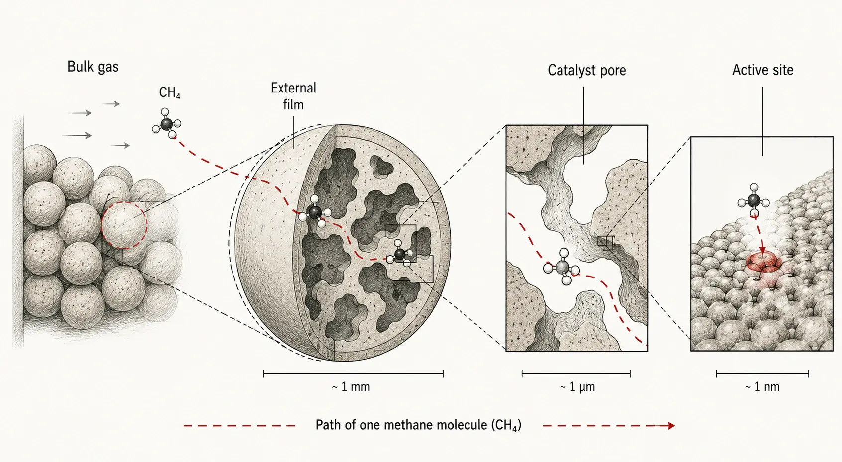
Figure 3 follows one methane molecule from the flowing gas to an active site inside the catalyst. This is probably the simplest way to understand why catalytic reactor modeling quickly becomes a multiscale problem. The methane molecule first moves with the bulk gas through the spaces between catalyst pellets. When it reaches a pellet, it must cross a thin region of gas close to the external surface. It then enters a pore that may be narrow, irregular, and far longer than the straight distance from the pellet surface to its center. Inside that pore, methane is surrounded by other molecules that are also moving, colliding, adsorbing, reacting, and leaving. Eventually the methane molecule may reach an active site where the surface reaction can begin. The products then have to move back through the pore before returning to the flowing gas. The chemical reaction itself may fit on one line of paper, but the physical journey needed to make that reaction happen stretches from the reactor scale down to pores and atomic-scale surface sites. This is where the simple idea of “reaction rate” begins to separate into chemistry and transport. A catalyst may have very fast chemistry, yet the reactor may still perform poorly if molecules cannot reach enough of the active surface. The next question therefore becomes surprisingly important: what happens if we make the catalyst chemistry faster than the molecules can move through the pellet?

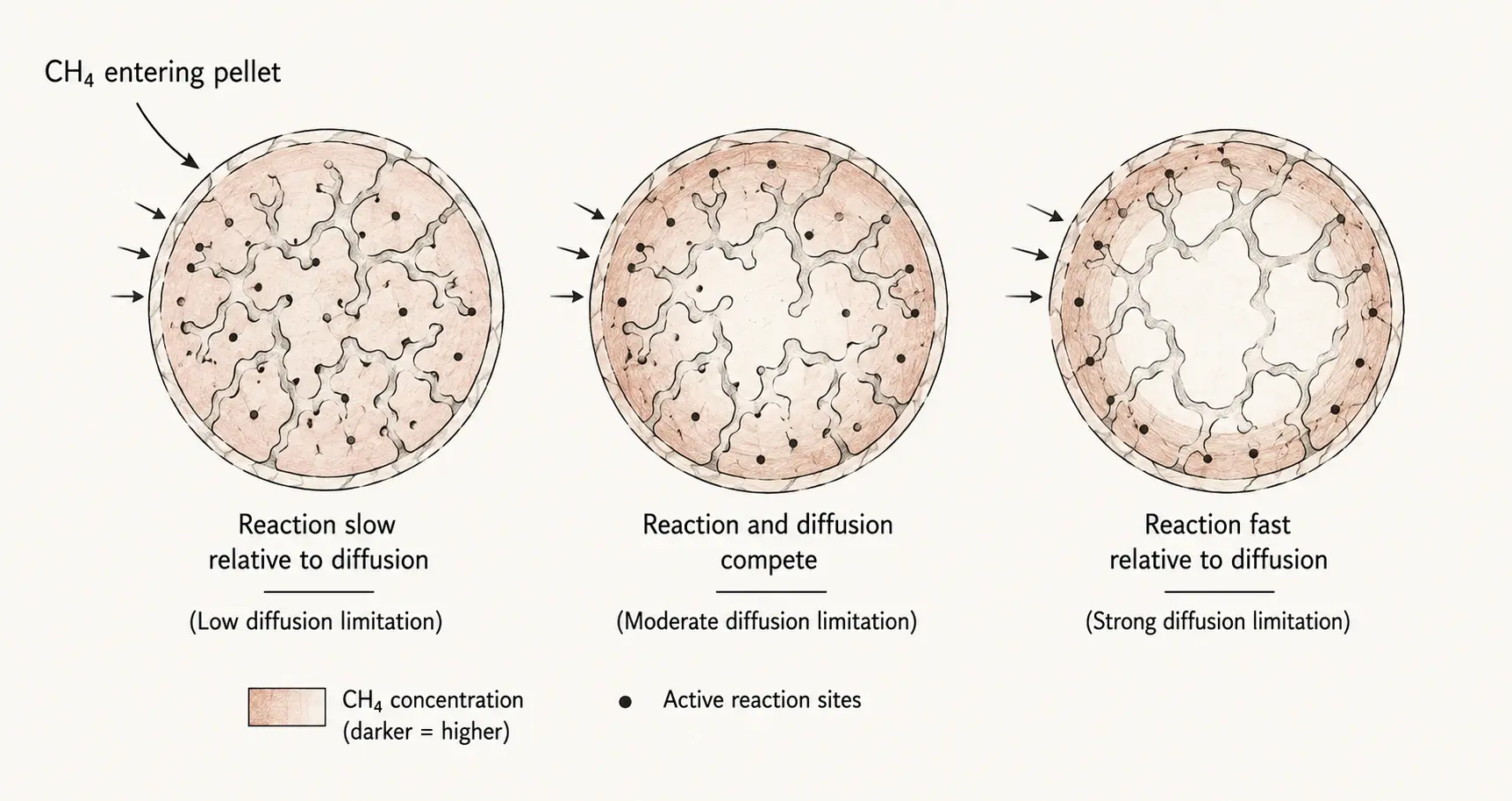
Figure 4 shows three pellets that are physically the same size, but the balance between reaction and diffusion changes from left to right. In the first pellet, molecules can move through the pore network faster than they are consumed, so methane concentration remains fairly similar throughout most of the pellet. Much of the internal catalyst can therefore participate in the reaction. In the middle pellet, reaction and diffusion begin to compete, so methane concentration falls as we move toward the center. In the third pellet, the reaction becomes so fast compared with diffusion that most methane is consumed near the outside before much of it can reach the center. The interior is still full of catalyst material, but some of that material is doing much less useful work. This is one of the most important ideas in catalytic reactor engineering because a better catalyst does not always produce an equally large improvement in reactor performance. If the surface chemistry becomes much faster but diffusion stays the same, transport becomes the new bottleneck. Engineers use the Thiele modulus to describe this competition between reaction and diffusion. For a simple first-order case:

$$\phi=R_p\sqrt{\frac{k}{D_{\mathrm{eff}}}}$$

A larger pellet gives molecules a longer distance to travel, a faster reaction consumes them more quickly, and lower effective diffusivity makes movement through the pore network more difficult. The equation therefore puts several physical ideas into one number, but the picture in Figure 4 is more important than memorising the equation.

Another useful quantity is the effectiveness factor:

$$\eta= \frac{\text{actual reaction rate of the pellet}} {\text{rate if the whole pellet were at surface conditions}}$$

The effectiveness factor simply asks how much of the theoretical catalyst activity we are actually using. If methane concentration and temperature are almost the same throughout the pellet, the whole pellet can contribute strongly, and the effectiveness factor may be close to one. If methane cannot penetrate deeply, the inner part contributes less and the effectiveness factor falls. This helps explain why catalyst design is more than finding a material with the fastest possible surface reaction. Pellet size, pore structure, porosity, diffusivity, and reaction rate all have to work together. A small pellet may reduce internal diffusion resistance, but smaller particles can also increase pressure drop through the reactor. A highly active catalyst may look excellent in a small laboratory experiment while transport limits its benefit in a larger reactor. Every time we improve one part of the system, another limitation may become more important. That is why catalytic reactor design is rarely about maximizing one property. It is about finding the right balance among chemistry, transport, heat transfer, pressure drop, and stability.

The Wall Is Hot, but Is the Catalyst Equally Hot?

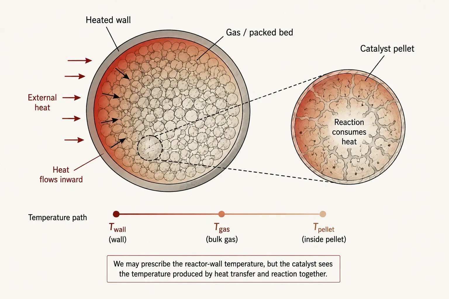
Biogas bi-reforming adds another layer because the reforming reactions need a large amount of heat. When we say that a reactor operates at 850°C or 900°C, it is easy to imagine that everything inside the reactor is at that same temperature. In reality, the furnace, reactor wall, flowing gas, catalyst surface, and center of the catalyst pellet can all have different temperatures. Heat has to travel from the heating source through the reactor wall, into the packed bed, through the gas, and into the catalyst where the reaction is taking place. At the same time, the reforming chemistry is consuming that heat. If the reaction becomes faster in one region, that region may remove heat more quickly and become cooler. The cooler temperature can then slow the reaction because reaction rates are strongly temperature dependent. Slower reaction reduces heat consumption, which can allow the temperature to recover. The reactor has, therefore, become a coupled system where reactions change temperature and temperature changes reactions. Thermodynamics is also changing with temperature, so the local temperature affects both the possible equilibrium state and the speed at which the reactor approaches it. This is why temperature cannot always be treated as a number that we simply type into the model. In a strongly endothermic reactor, temperature is one of the things the model must calculate.

Figure 5 makes this point without requiring a complicated heat-transfer equation. The reactor wall is heated from outside, heat moves inward through the packed bed, and the catalyst pellet receives only the heat that actually reaches it. The temperature at the wall can therefore be different from the temperature in the gas, and both can be different from the temperature inside a reacting pellet. This matters because a kinetic rate constant calculated at the wall temperature may seriously overpredict the real catalyst rate if the pellet itself is cooler. The problem becomes even more important as reactor diameter increases because heat may have a longer distance to travel from the wall toward the middle of the bed. The catalyst near the wall may therefore experience a different thermal environment from the catalyst near the reactor center. The same is true along the reactor length because the inlet gas, intermediate gas, and outlet gas have different compositions and heat requirements. A single number called “reactor temperature” may therefore hide a great deal of useful information. For some systems, that simplification is perfectly acceptable, while for others it is not. The model should only become more complicated when those differences actually affect the engineering decision. This idea will become important again when we decide whether a simple reactor model is enough or whether full CFD is really needed.

One Pellet Is Not a Reactor

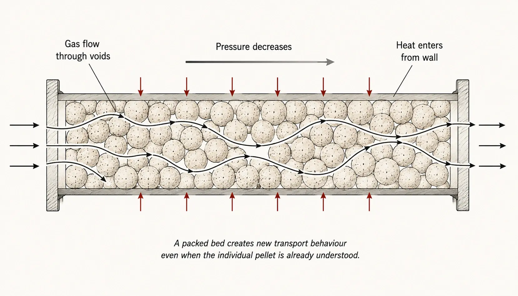
Suppose that we somehow understand one catalyst pellet perfectly. We know its kinetic behavior, pore diffusion, heat transfer, and effectiveness factor under any condition. We might think that building the reactor model is now simply a matter of multiplying that pellet by a few hundred thousand. Figure 6 shows why that is not correct. Once many pellets are packed into a tube, the gas must move through irregular spaces between them rather than through a clear straight channel. Some flow paths are easier than others, and the gas bends repeatedly as it travels around the particles. The packed bed creates resistance, so pressure decreases from the inlet toward the outlet. Heat also has to move from the reactor wall through a mixture of gas, solid particles, and contact points between particles. The bed near the wall can have a different packing structure from the bed farther inside, which can change both flow and heat transfer. At the same time, gas composition changes because methane is being consumed and hydrogen and carbon monoxide are being produced. Density, viscosity, thermal conductivity, and other properties can therefore change as the gas moves through the reactor. A pellet near the inlet does not experience the same environment as one near the outlet. The reactor has created new transport behavior that was not present when we studied one isolated pellet.

At this scale, conservation equations become the bridge between local catalyst behavior and complete reactor performance. For species (i), a general species balance can be written as

$$\frac{\partial(\rho Y_i)}{\partial t} +\nabla\cdot(\rho\mathbf{u}Y_i) =-\nabla\cdot\mathbf{J}_i+S_i$$

There is no need to be intimidated by the notation. In plain language, the equation says that the amount of a chemical species in a small region changes because the species can flow in or out, diffuse in or out, and be created or destroyed by chemical reactions. Similar balances are written for momentum and energy. Together, these equations allow us to calculate velocity, pressure, temperature, and composition through the reactor. The difficulty is that an industrial reactor can contain far too many pellets and pores to resolve every physical detail directly. Engineers therefore replace some small-scale details with effective properties or correlations. Pressure drop, effective thermal conductivity, dispersion, permeability, and other quantities may come from simplified models or experiments rather than direct calculation from every microscopic feature. We have again reached the same pattern: fundamental conservation laws form the backbone of the model, but practical reactor prediction still requires information from smaller scales. Solving the conservation equations perfectly does not help if the kinetic or transport information supplied to them is wrong. This is why a larger simulation is not automatically a better prediction.

Do We Really Need CFD?

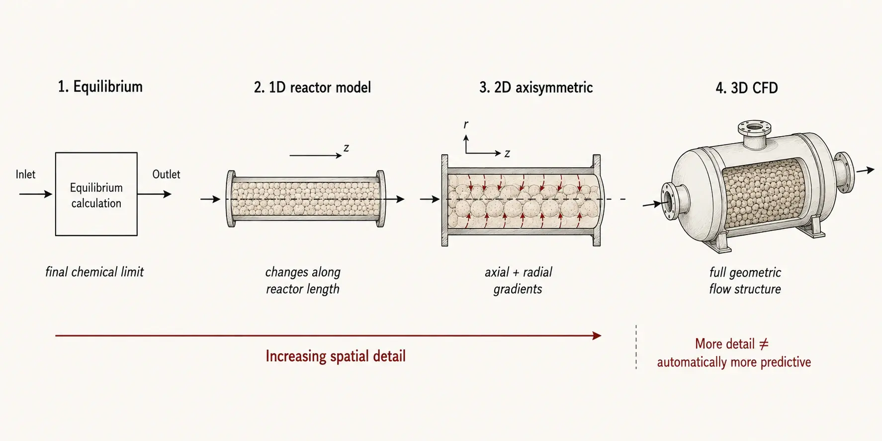
Figure 7 shows four ways to represent the same reactor, and the important point is that each level answers a different question. An equilibrium calculation may be enough if we only want to know the final chemical limit under a chosen temperature, pressure, and feed composition. A one-dimensional model adds the reactor length, so it can predict how temperature, pressure, and composition change as the gas travels from inlet to outlet. A two-dimensional axisymmetric model can also resolve radial changes from the reactor wall toward the center. Full three-dimensional CFD becomes useful when the actual geometry creates important nonuniform flow, asymmetric heating, complex inlet or outlet manifolds, structured catalyst regions, or internal hardware. The natural temptation is to assume that moving from left to right on Figure 7 always makes the answer better. That is not necessarily true. A simple one-dimensional model using reliable kinetics and heat-transfer information can sometimes be more useful than an enormous CFD model using uncertain physical inputs. A CFD solver may calculate the equations on millions of cells with excellent numerical accuracy, but it cannot know whether the kinetic rate, catalyst diffusivity, thermal conductivity, or boundary condition supplied by the engineer is correct. More spatial detail only adds value when that extra spatial detail represents physics that actually matters to the design. The goal is therefore not to build the most complicated model possible. The goal is to build the simplest model that still contains the important physics.

This idea also changes how we should think about uncertainty. Suppose a detailed model predicts methane conversion of 87.3%. The decimal point may make the result look very precise, but perhaps the activation energy is uncertain, the catalyst diffusivity is only estimated, and the real wall temperature is not known perfectly. In that situation, 87.3% is only the answer for one particular set of assumed inputs. A small change in one important parameter might move the prediction to 84%, while another change might move it above 90%. Sensitivity analysis helps us discover which uncertain inputs matter most. If conversion changes strongly when the kinetic parameters change but barely changes when axial dispersion changes, better kinetic experiments may be more useful than a finer mesh. If the result is very sensitive to pellet diffusivity, then catalyst characterization becomes more important. If the H₂/CO ratio changes strongly with heat-transfer conditions, then temperature measurements deserve more attention. This is one of the most practical jobs of a good reactor model: it should tell us not only what the reactor may do but also what we still need to know. Sometimes the most valuable result from a simulation is not another contour plot but the discovery that one poorly known parameter controls the whole prediction.

The Model Predicts 84%. Is It Correct?

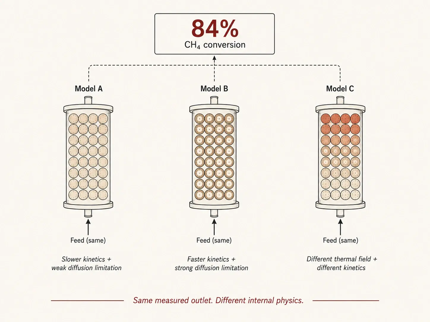
Now we arrive at one of the most interesting parts of the problem. Imagine that we finally build the reactor and measure 84% methane conversion at the outlet. Our model also predicts 84%, so it is natural to feel that we have succeeded. Figure 8 shows why we should be careful. Model A may use slower intrinsic kinetics and assume that diffusion through the pellet is easy. Model B may use much faster kinetics but also much stronger internal diffusion limitation. Model C may use a different temperature field together with a different set of kinetic parameters. All three can potentially give the same 84% outlet conversion even though the physics inside each model is different. If all we measure is the final methane conversion, we cannot easily know which explanation is correct. The model may therefore give the right answer for the wrong reason. This is not simply a mathematical curiosity because the problem becomes visible when operating conditions change. Increase the pellet size, change the flow rate, raise the pressure, change the amount of steam, or alter the heating condition, and the three models may suddenly predict very different reactor behaviors. A model that only reproduces the condition where it was fitted is not necessarily predictive.

This is why good experiments should do more than provide numbers for fitting. They should help us separate one physical explanation from another. Changing pellet size can help reveal whether internal diffusion is important. Changing flow rate can expose external mass-transfer effects or residence-time limitations. Measuring temperature inside the bed gives information that outlet conversion alone cannot provide. Pressure-drop measurements can test the packed-bed flow model without depending on reaction kinetics. Carefully designed kinetic experiments can reduce transport limitations so that the intrinsic catalyst behavior is easier to identify. Transient experiments can reveal response times that disappear in steady-state measurements. Each experiment should ideally remove one possible wrong explanation. In this way, modeling and experiments become partners rather than separate activities. The model tells us what we do not know, and the experiment is designed to reduce that uncertainty. A good validation program therefore does not ask only, “Did the model match the experiment?” It asks the more difficult question, “Did the model match the experiment for the correct physical reason?”

Come Back After 1,000 Hours

Even if we solve all of these problems at the beginning of operation, the reactor can still change with time. Carbon formation is especially important in methane reforming because carbon can form through several chemical routes. Two simple reactions that illustrate the problem are methane cracking,

$$\mathrm{CH_4\rightleftharpoons C+2H_2}$$

and the Boudouard reaction,

$$\mathrm{2CO\rightleftharpoons CO_2+C}$$

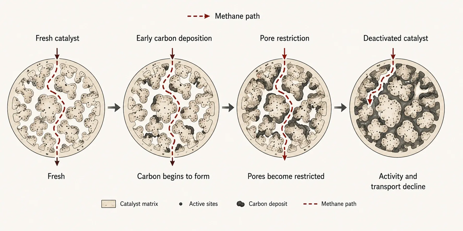
although the real carbon chemistry on a catalyst can be much more complicated. Thermodynamics can help us identify conditions where solid carbon is favorable, but it does not automatically tell us how fast carbon appears or what form it will take. Carbon may begin as small deposits on the catalyst surface, grow along pore walls, block active sites, and eventually restrict transport through the pore network. Figure 9 shows the important idea: the catalyst itself is changing. At the beginning, methane can travel deep into the pore network and reach many active sites. As carbon builds, some paths become narrower and some sites become covered. Later, methane may reach only part of the catalyst that was originally available. The reactor at hour 1 is therefore not exactly the same physical reactor at hour 1,000, even if the steel vessel and operating settings have not changed.

Once the catalyst changes, many parameters in the original model may also change. Effective diffusivity can fall because pores become restricted. The accessible catalytic area can decrease because carbon covers active sites. Local reaction rates change, which changes gas composition and temperature, and those changes can then affect further carbon formation. Catalyst aging can therefore create another feedback loop. Other deactivation mechanisms such as sintering, poisoning, oxidation-state changes, or structural changes can make the problem even more difficult. A reactor model that predicts startup performance very well may still have little ability to predict long-term catalyst life. This matters because the best reactor is not necessarily the one with the highest methane conversion on the first day. A design with slightly lower initial conversion may be much more valuable if it remains stable for much longer, requires less regeneration, has a lower pressure drop, or uses less heat. Reactor design is therefore a balance among conversion, selectivity, heat demand, pressure drop, catalyst use, carbon resistance, lifetime, and operating flexibility. This is where the idea of a single “best” operating point often becomes misleading. The best design depends on what the reactor must achieve over its entire useful life.

Where Can Neural Operators Actually Help?

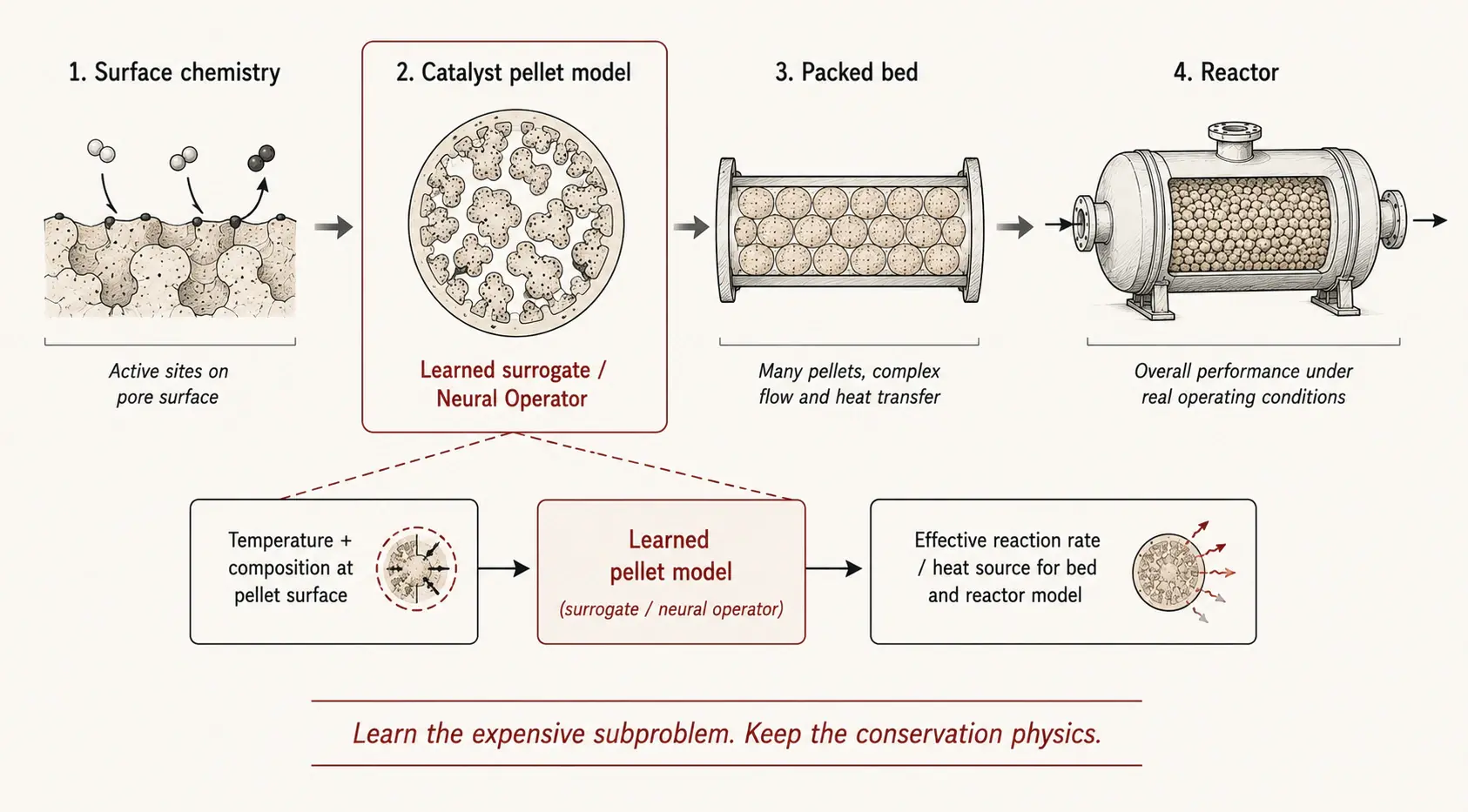
After following the reactor from equilibrium all the way down to catalyst pores and then back up to the full packed bed, another problem becomes clear: some of these calculations can be very expensive. A detailed surface-chemistry model may contain many reactions and intermediate species. A pellet model may need to solve reactions, diffusion, and heat transfer again and again as temperature and composition change along the reactor. A full reactor simulation may then have to repeat those smaller calculations thousands or millions of times. If we want to optimize the reactor, study uncertainty, or test thousands of operating conditions, computational cost can become a serious barrier. This is where Neural Operators or other learned surrogate models can become useful, but the role needs to be chosen carefully. Instead of asking an AI model to replace the entire reactor, we can ask it to learn one expensive repeated subproblem. Figure 10 shows an example where the pellet calculation is replaced by a fast-learned model. The reactor still supplies local temperature and composition, while the learned pellet model quickly returns the effective reaction rate and heat source needed by the larger reactor calculation. Mass conservation, energy conservation, thermodynamics, and the overall reactor structure remain in place. The learned model is used to reduce computational cost, not to remove the physics we already understand.

This approach also makes the limitations of machine learning easier to see. A learned model can only reproduce behavior represented in the data or simulations used to train it. If the original pellet simulations ignored carbon formation, the learned model will not suddenly discover long-term carbon deposition by itself. If the training data covered only a narrow temperature range, predictions far outside that range may not be reliable. If the underlying kinetics are wrong, a fast surrogate will simply reproduce the wrong kinetics faster. The useful role of Neural Operators is therefore not to rescue an incomplete physical model. Their value is in accelerating parts of a well-defined model that are already understood but expensive to solve repeatedly. This distinction matters because it keeps the engineering question in the correct order. First decide which physics is needed, then decide how that physics should be modeled, and only after that decide whether part of the calculation is expensive enough to justify a learned surrogate. AI becomes one computational tool inside the reactor model rather than the reactor model itself. That approach is less dramatic, but it is much more useful for engineering.

So, Did We Predict the Reactor?

We started with a reactor that looked simple: methane, carbon dioxide, and steam went in, heat entered through the wall, and hydrogen-rich syngas came out. Thermodynamics first told us where the chemistry wanted to go, but it could not tell us how long the journey would take. Kinetics gave the chemistry a clock, but the kinetic parameters introduced experimental and molecular information into our supposedly first-principles calculation. Following one methane molecule showed that even perfect surface chemistry could not help if reactants could not reach the active sites. Pellet diffusion then explained why a faster catalyst can eventually become limited by transport. Heat transfer showed that the catalyst temperature is not simply the temperature we choose for the reactor wall. Packing many pellets together created pressure drop, irregular flow paths, and new heat-transfer behavior. Reactor-scale equations allowed us to connect these effects, but they also required effective properties and closures for physics that could not be resolved directly. Increasing the model from equilibrium to 1D, 2D, and full CFD added spatial detail, but not automatic certainty. Validation then showed that several physically different models can reproduce exactly the same outlet conversion. Catalyst aging made the problem harder again because the material doing the chemistry changes with time.

After all of this, the answer to our opening question is neither a simple yes nor a simple no. We can predict a great deal about a biogas bi-reforming reactor using fundamental physics, thermodynamics, transport theory, reaction kinetics, and numerical methods. Some parts of the reactor can be calculated with high confidence, while other parts depend strongly on experimental kinetic data, catalyst structure, transport properties, correlations, boundary conditions, and assumptions. The useful goal is therefore not to claim that a reactor is completely “first principles” simply because it contains many equations. A better model is one where we know which pieces come directly from physical laws, which pieces come from measurements, which pieces are approximations, and which uncertainties control the final engineering decision. That understanding tells us where a simple model is enough, where a detailed simulation is worth the cost, and where another experiment will teach us more than another million computational cells. It also tells us where faster tools such as Neural Operators can help without hiding the physics that matters. The strongest reactor model is not the one that looks most complicated or produces the most colorful contour plot. It is the one that continues to explain the reactor when conditions change. In the end, perhaps the most useful question is not whether we can predict a biogas bi-reforming reactor completely from first principles but something more practical: Which parts can we predict from physics, which parts must we measure, and which parts actually control the design?

M² Engineering

At M² Engineering, this is how we approach difficult reactor problems: start with the physics, understand where the uncertainty really comes from, and only then decide how much numerical complexity is justified. Whether the challenge is catalytic reforming, reaction–diffusion inside porous media, heat transfer through packed beds, reactor-scale CFD, or reduced-order modeling with Neural Operators, our focus is not on producing the most complicated model. It is about building the model that gives the most useful engineering answer. If you are working on a reactor where chemistry, transport, heat transfer, and computation are tightly coupled, M² Engineering can help turn that complexity into a practical design and decision-making framework.

M2 Engineering